The sampling distribution is one of the most important concepts in inferential statistics, and often times the most glossed over concept in elementary statistics for social science courses. This article will introduce the basic ideas of a sampling distribution of the sample mean, as well as a few common ways we use the sampling distribution in statistics. When we conduct a study in psychology, this almost always includes taking a sample and measuring some aspect or characteristic about that sample. While we assume that a large enough sample will represent the population enough to make statistical inferences, there can be natural variation between two different samples taken from the same population. This sampling variation is random, allowing means from two different samples to differ. The sampling distribution of the sample mean models this randomness.
Definition In statistical jargon, a sampling distribution of the sample mean is a probability distribution of all possible sample means from all possible samples (n).
In plain English, the sampling distribution is what you would get if you took a bunch of distinct samples, and plotted their respective means (mean from sample 1, mean from sample 2, etc.) and looked at the distribution. Except a “bunch of” samples is really ALL samples, and this distribution can be used to infer the probability you got a specific mean from any sample. That last sentence was a bit confusing right? Let’s look at an example to clarify.
Example Say you are curious about the average height for a college student at College X. You then go to four random classrooms on campus, and measure all of the students’ heights in the class. Each classroom has one sample mean, but they slightly differ. For example, the four means from the four samples could be as follows:
Class 1 mean height → 67 inches
Class 2 mean height → 70 inches
Class 3 mean height → 66 inches
Class 4 mean height → 68 inches
If you plot these points, it looks like this:
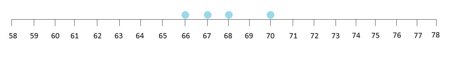
Not really much of a distribution, right? Now let’s say we went to a lot more classes, took students’ height measurements, calculated their means and added them to our previous four means. It could look something like this:
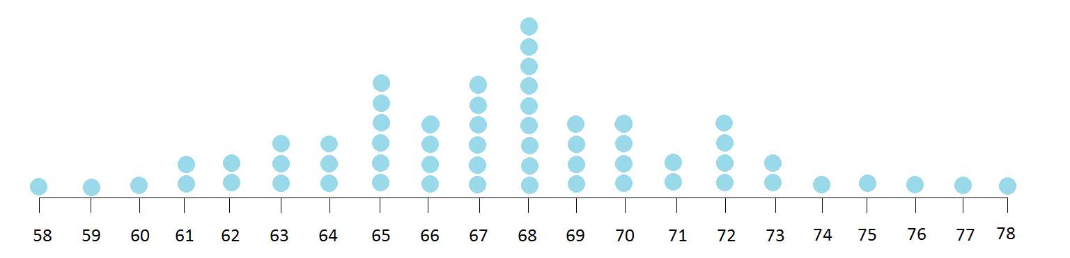
In fact, if we somehow were able to take ALL samples from the entire population of college students at College X, you would see something like this:
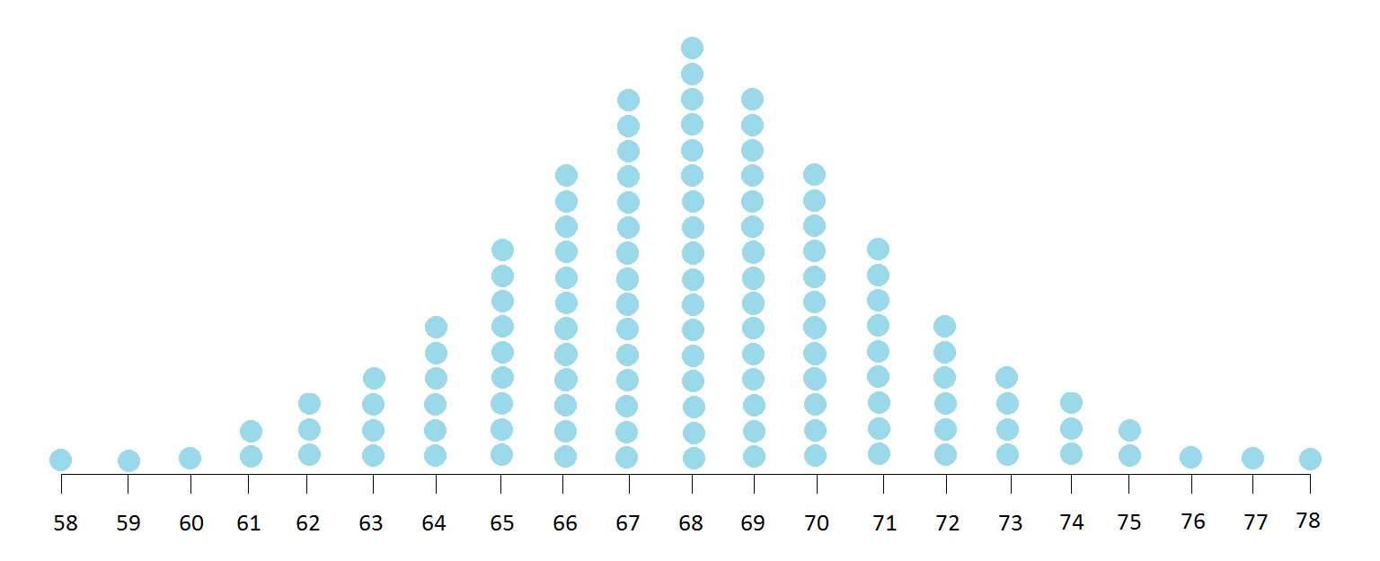
This last distribution is the sampling distribution of sample means. It is a distribution created by every possible mean from every possible sample. And if you already noted that it resembles a normal distribution, well then you would be correct! According to the Central Limit Theorem, if the samples used to create each mean of the distribution are large enough, the sampling distribution of the mean of any independent random sample will be normally distributed, even if the population distribution is not perfectly normal.
The sampling distribution of the sample mean is very useful because it can tell us the probability of getting any specific mean from a random sample. Put more simply, we can use this distribution to tell us how far off our own sample mean is from all other possible means, and use this to inform decisions and estimates in null hypothesis statistical testing.
Standard Error of the Mean One aspect we often use from the sampling distribution in inferential statistics is the standard error of the mean (noted as SE, or SEM). The SEM is a hard concept to grasp for many individuals, but once you understand the sampling distribution it’s actually quite simple.
The SEM is the standard deviation of the sampling distribution, calculated by dividing the standard deviation by the square root of the sample size (n) for a given sample.

We often use elements of the standard error of the mean when we make inferences in statistics. For example, the t statistic for an independent samples t test uses the SEM as the denominator.
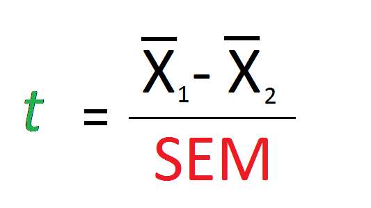
In this sense, the numerator of this t statistic is the difference in means between group 1 and group 2, and the denominator is the standard deviation of all possible means from all possible samples. What the t value then represents is how different the means of group 1 and group 2 are in standard units.
Further, to get a confidence interval of your mean estimate for an independent samples t test, you also use the SEM.
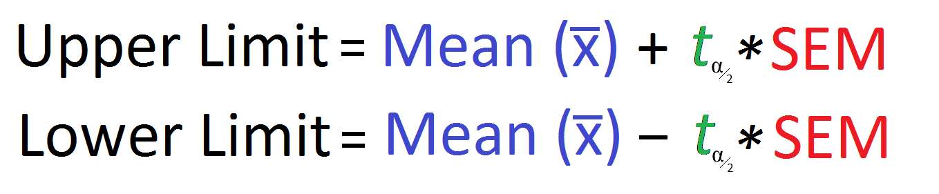
Using the SEM allows you to calculate a confidence interval of the mean estimate because it brings in the element of variability in any given sample mean. The larger the standard deviation of the sampling distribution is, the larger your confidence interval will be.
Conclusion The sampling distribution of the sample mean represents the randomness of sampling variation of sample means. This distribution is an integral part to many of the statistics we use in our everyday research, though it doesn’t receive much of the spotlight in traditional introductory statistics for social science classrooms.
If you would like to learn more about sampling distributions, visit the follow websites which talk more about sampling distributions.
[1] https://www.khanacademy.org/math/probability/statistics-inferential/sampling-distribution/v/sampling-distribution-of-the-sample-mean
[2] http://stattrek.com/sampling/sampling-distribution.aspx
[3] http://www.psychstat.missouristate.edu/introbook/sbk19.htm
[4] http://www.vassarstats.net/textbook/ch6pt1.html