From my interactions with undergraduate students, it seems that even though these definitions are easy to recite, they are difficult to be integrated into a comprehensive whole. I hope here to show how to conceptually integrate them into a cohesive picture.
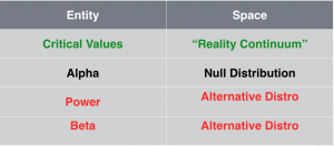
Everything begins with reality: the “Reality Continuum”
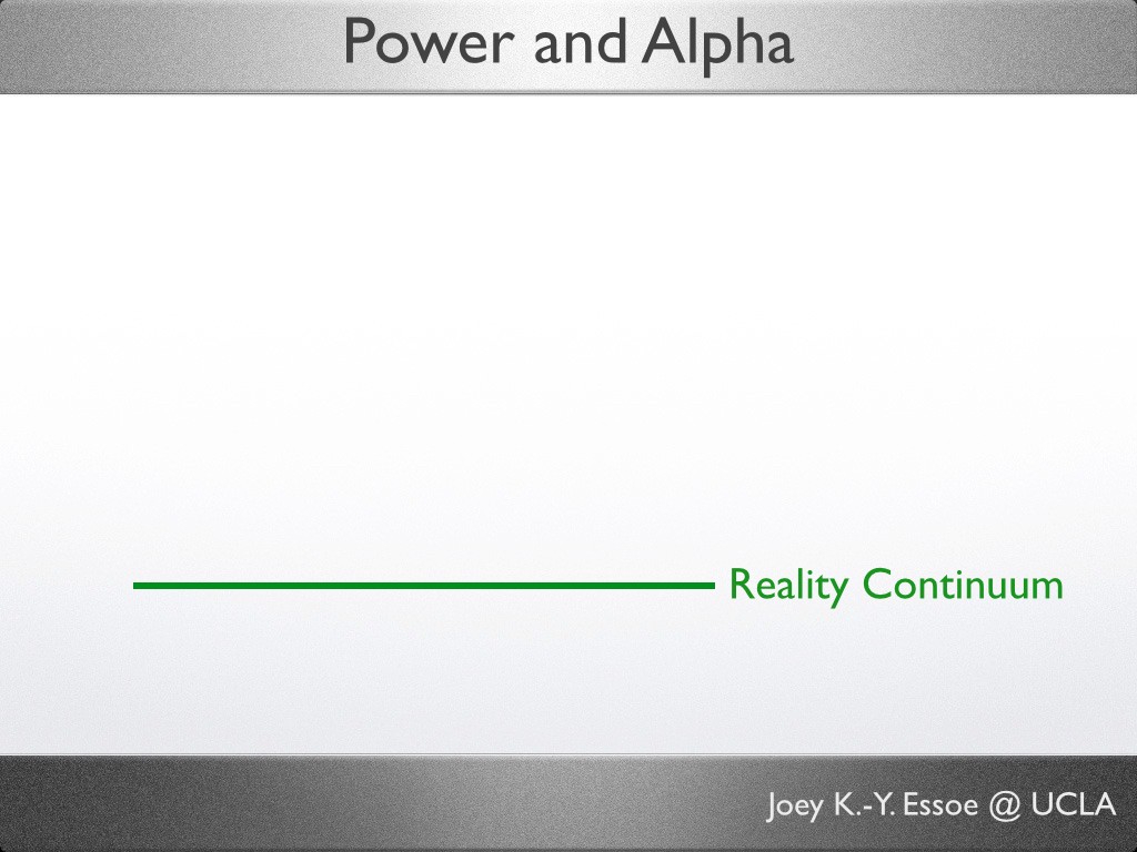
I call this green line “Reality Continuum” (rather grand, no?) because you will take your ideas, and do a reality check against it via data analysis (within the traditional statistical framework–it is definitely NOT the only framework on the market, but I digress).
This continuum extends from negative infinity to positive infinity. Each point on this line depicts a potential value of some statistical entity about the “populations” you are interested in. What that entity is depend on the statistical tests you are conducting. For example, each point on this continuum could be a series of Z values (as in a Z tests), means (single sample t-test), mean differences (paired sample t-tests), or the differences of the means (independent sample t-test), etc.
Upon this continuum we will draw certain distributions. The most common of all are the normal distribution (e.g. Z- and t-distributions). While this post shows only normal distributions, there are statistical entities that follow non-normal distributions (e.g. the F- and Chi Square distributions are positively skewed) — nearly everything in this post can be applied to all of these distribution except that they do not support two-tailed hypothesis testing.
Distributions in General
- The famous “bell-curve” is NOT made of the residences from the Reality Continuum, but the probability (comparative frequencies) of these residences. Therefore, the height of a given portion within the curve represents the likelihood of “drawing” the corresponding value during a random selection process.
- It is not even a curve. The distribution describes the area UNDER the curve! I often think that the “bell-curve” title has done this concept a disservice as it mislead people to think of it as a line. The line merely serves as a boundary for the area beneath.
- All the distributions mentioned here sum to 1. Meaning everything under the curve sums to a 100% probability.
Properties of a Normal Distribution
- Symmetrical (its left side looks like the mirror image of the right side)
- Uni-modal (only has 1 peak/hump)
- Asymptotically (infinitely approaches zero, but never quite getting there)
The Null Distribution
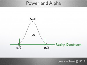
Based on your research idea, you form a set of null and alternative hypotheses. Under the assumption of normality, you will draw a null distribution that centers on the null (non-interesting/default) mean.
* All the concepts below, until the “Alternative Hypothesis” Section, are related to the null distribution.
Alpha Level (α)
Since everything operates on probability in the tradition hypothesis testing framework, you need to decide what is the acceptable probability for Type I Error: α is simply that.
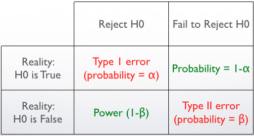
Type I Error (Def.):
“The incorrect rejection of the null hypothesis.” Or
“Rejecting the null hypothesis while it is true.”
Alpha (Def.):
“Acceptable probability for Type I Error to occur.” Or
“Acceptable probability for rejecting the null hypothesis while it is true.”
Type I Error is an event, and Alpha is the probability for that event’s occurrence.
Alpha is a portion of the null distribution (recall that the distribution is not the curve, but the area under the curve).
If α=.05, Alpha would take up .05 of the null distribution at the extreme(s)–the 5% that is farthest away from the center.
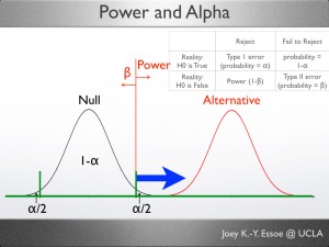
When the hypothesis is non-directional/two-tailed (e.g. dogs are different from cats), as shown in the image here, each tail gets half of alpha, so α/2=.025, or 2.5%.
When the test is directional/one-tailed (e.g. dogs scored lower than cats), the area of α would be placed at the relevant tail (in the example, it would be on the low end).
Alpha (α) is not calculated, but is decided upon (by researchers, and based on consensus that vary across scientific fields) . Most social sciences use the α = .05 guideline, much higher than the physical sciences. This 5% guideline was an entirely arbitrary decision made by some very brilliant people* (consider them the “gods of statistics in whom we lay our faith”).
* A treat for you history buffs: check out “On the origins of the. 05 level of statistical significance” by Drs. M. Cowles and C. Davis (1982). Dr. Carl Anderson’s blog post (“What’s the significance of 0.05 significance?” on p-value.info) stated that Cowles and Davis “describe a fascinating extended history which reads like a Whos Whos of statistical luminaries.”
What does an alpha level of .05 mean for Type I Error?
It means that we (of the social sciences) accept that 1 out of 20 times when we reject the null hypothesis, we are wrong. Alternatively and logically, for every 20 social science results we publish, 1 of them is a false positive.
Please do not be (too) alarmed, these are not experiments upon whose results the FDA would decide whether an antidepressant is safe to take–those type of experiments follow different guidelines and protocols.
One of the reasons why the acceptable false positive rate is set at 5% is this: unlike other branches of sciences, social sciences work with data that contain more variability. The behaviour/state of your psyche is more complex and unpredictable than, say, your kidneys.
However, it is very important to keep this in mind before making important life-style changes or life decisions based on these type of research (and don’t get me started on the misinterpretation of correlational relationships, see Adi Jaffe’s post on the topic.).
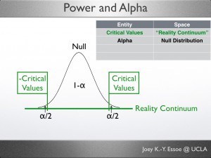
Critical Values
Once we have decided on a alpha level, we can use it to locate the critical value on the Reality Continuum. A few different ways to think about Critical Value are provided below.
Critical Value (Def.):
“Critical Value is the value beyond which the portion (%) of the null distribution sums to α.” Or
” Critical Value(s) is the cut-off value at which the null distribution is divided to two parts, α and 1-α.” Or
“Beyond the critical value(s) lays a portion of the null distribution whose area = α.”
In a 2-tailed test (shown here) there will be 2.5% on each side of the curve, so there would be two critical values, one positive (above the mean) and one negative (below the mean). In a 1-tailed test, there would only be 1 area and 1 critical value.
So to reiterate,
- Alpha is a probability that you would use to locate a particular resident on the Reality Continuum–that resident is the Critical Value.
- Under the null hypothesis, the probability of finding something as extreme as, or more extreme than the critical value(s) is 5% (α).
Tangent on p-Values
p-values and Critical Value are really two sides of the same coin. While critical value represents numbers on the Reality Continuum based on α, a p-value represents a probability itself that describe the observed test statistics.
For example, if you run a t-test and find that the t-value is 8, the correspond p-value tells you, “What is the probability of obtaining a t-value as extreme as 8 if the null hypothesis is true.” So if the p-value is less than α, you would conclude that your test is statistically significant.
The p-value of the critical value is always α.
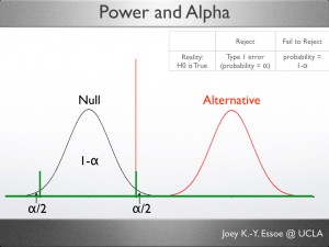
The Alternative Distribution
So far, everything is happening around the null distribution, either on the reality continuum or the area under the curve. Now we will extend the reality continuum and introduce our new friend, the alternative, or comparison, distribution. It is also a probability distribution, centered around the hypothesized mean. The distance between the null and hypothesized means represents how different the distributions are.
Traditionally, textbooks draw the alternative distribution to the right (higher value) of the null distribution. I suspect that this is because it is more intuitive to think of a treatment/experimental condition “improving” the outcome variable. However, a treatment could just as easily decrease the outcome (e.g. reducing depression symptoms, etc).
Power + Beta = Alternative Distribution (=1)
The alternative distribution can be thought of as being made of two parts: Beta and Power. Since the entire alternative sums to 1, Beta + Power = 1, and Power = 1-Beta.
Type II Error (Def.):
“Failing to reject the null hypothesis when it is false.” Or
“Incorrectly retaining the null hypothesis.”
Beta (Def.):
“The probability for Type II Error to occur.” Or
“The portion of the alternative distribution that falls on the non-rejection side of the critical value.”
Power (Def.):
“The probability of rejecting the null hypothesis while it is false.” Or
“The probability of correctly rejecting the null hypothesis.” Or
“The portion of the alternative distribution that falls on the rejection side of the critical value.”
(Noted by a blue arrow in the figure.)
Type II Error is an event, and Beta is the probability for that event’s occurrence.
Why is Beta and Power so confusing?
The tricky part about Power and Beta is this: While they live on the alternative distribution, their values depend on the critical value, which lives on the null distribution.
The graph shows that the green line that marks our critical value is also the location in which the alternative distribution is split into Beta and Power (red extension of the line).
You might have heard that Beta and Power depends on Alpha, that is true. All else being equal, when Alpha changes the critical value also change. Therefore, the split point on the alternative distribution that divides it into Beta and Power would change.
Last but not least: Important Distinctions
Alpha, Power, and Beta are probabilities. Type 1 Error and Type II Errors are events.
The “Who lives where” chart
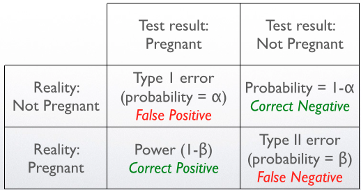
Summary and Analogy
An often used, but very apt way of understanding the above table is the analogy of pregnancy test:
How Power relates to…
I will demonstrate how power changes when the other parameters change. Most likely a using video blog post.
Credit
This post was edited by our new blog master, Tawny Tsui. See her posts here.
Reference
Cowles, M., & Davis, C. (1982). On the origins of the. 05 level of statistical significance. American Psychologist, 37(5), 553.
Thumbnail picture from https://ih0.redbubble.net/image.248946736.4291/flat,800×800,070,f.u1.jpg